Lecture 9

Andreas Moshovos

Spring 2007

The C Switch Statement

In this section we will be implementing in assembly a C switch statement. Let’s us use a specific example. Assume that we somehow know that a integer variable p takes values in the range of 0 through 7. The code that we are interested in is:

int av;
int bv = 0x12345678;
int cv = 0x11223344;

int p = some value;

switch (p)
{
   case 0: a = b + c; break;
   case 1: a = b - c; break;
   case 3: a = b; break;
   case 7: a = c; break;
   default: a = 0;
}

The default statement is executed in all cases that are not explicitly referred by a “case” statement. Accordingly, our switch statement is equivalent to the following:

switch (p)
{
   case 0: a = b + c; break;
   case 1: a = b - c; break;
   case 3: a = b; break;
   case 7: a = c; break;
   case 2:
   case 4:
   case 5:
   case 6:
                a = 0;
}

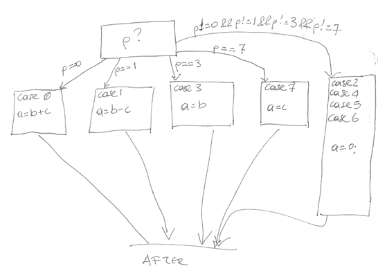
If we were to draw a control flow diagram for this code it would look as follows:

Notice that the first box, is a decision box with many different branches. There are five different possible targets out of this box. We can synthesize this behavior using several if-the statements. So in C we could implement the switch also as:

if (p == 0) goto case0;

if (p == 1) goto case1;

if (p == 3) goto case3;

if (p == 7) goto case7;

goto casedefault;

case0:

a = b+c;

goto done;

case1:

a=b-c;

goto done;

case3:

a = b;

goto done;

case7:

a = c;

goto done;

casedefault:

a = 0;

done:

You should now be able to convert that into assembly using branches. Assume for this code that p is in d0:

cmp.l #0, d0

beq case0

cmp.1 #1, d0

beq case1

cmp.l #3, d0

beq case3

cmp.l #7, d0

beq case7

bra casedefault

case0

…

bra after

case1

…

bra after

case3

…

bra after

case7

…

bra after

casedefault

…

after

In the worst case scenario we will have to go through all comparisons to reach the “bra casedefault” for this simple switch statement. What if our switch statement had 50 cases? It would be nice if there was a faster way of implementing multi-way branches. And fortunately there is, we can use a jump table. A jump table is an array with an element for each possible value of the switch variable (p in our case). The value of each jump table element is an address. This is the address where the code for the corresponding case statement lies in memory. Our assembly implementation with thus have a data segment containing the jumptable with appropriate values. The code will start by using p as an index to read an element from the jumptable (read jumptable[p]). The next step would be to use an appropriate control flow instruction so that execution continues at the address pointed to by the jumptable[p] element.

In pseudo-code notation, out implementation will look like this (note this will not work in C):

unsigned int jumpTable[8] = {case0, case1, defaultcase, case3, defaultcase, defaultcase, defaultcase, case7};

goto jumpTable[p];

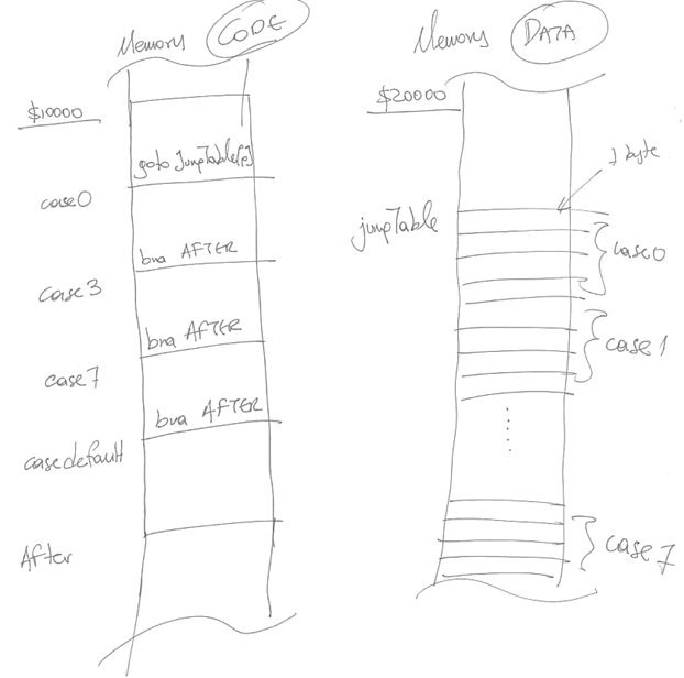
Here every element of jumpTable[] is an address to a piece of code that implements the corresponding case. For example jumpTable[1] contains the address “case1” which should be a label placed at the beginning of the block of instructions that implement case1. JumpTable[2] is “defaultlabel” because when p is 2 we want the code implementing the default case. In memory my code and jumptable will look as follows:

Here’s the implementation in assembly. The embedded comments explain the logic behind this code. This is by no means the best implementation of each required step. We will progressively see better ways of calculating arrays indexes and of accessing memory variables.

org $20000

; the jumpTable follows, each element is a code label that will be defined later on

jTable dc.l case0,case1,case2,case3,case4,case5,case6,case7

va dc.l $0 ; variable a

vb dc.l $12345678 ; variable b

vc: dc.l $11223344 ; variable c

vp: dc.l $3 ; variable p

org $20000

start

; we want to read element jTable[p]

; this is at address jTable + 4 x p in memory since each jTable element is four bytes long

movea.l #jTable, a0 ; [a0] = &jTable[0] the address where the jTable array starts at in memory

; notice the different between #vp and just vp. The first is the value of label vp

; this is $20000 in our case. Just vp refers to the memory contents at vp

; this would be case0 in our case

move.l vp, d0 ; read the value of variable p into the d register

add.l d0, d0 ; [d0] = 2 x p

add.l d0, d0 ; [d0] = (2 x p) + (2 x p) = 4 x p

adda.l d0, a0 ; [a0] = jTable + 4 x p

movea.l (a0), a0 ; [a0] = jTable[p]

jmp (a0) ; [pc] = jTable[p] (see discussion below)

; continue execution at the label contained in jTable[p]

case0

move.l vb, d0 ; va = vb + vc

add.l vc, d0

move.l d0, va

bra after ; this implements the “break”, i.e., continue execution after the switch (after is label)

case1

move.l vb, d0

sub.l vc, d0

move.l d0, va ; va = vb – vc

bra after

case3

move.l vb, d0

move.l d0, va ; va = vb

bra after

case7

move.l vc, d0

move.l d0, va ; va = vc

bra after

case2

case4

case5

case6

clr.l va

after

Note regarding the JMP instruction syntax: I consider the syntax of the JUMP instruction *confusing*. Here’s why. In our code we used JMP (a0). Based on our previous discussion (see lecture on arrays) when the “(a0)” is used as an operand then this is interpreted as Mem[ [a0]]. Not so for the JMP instruction. JMP uses the effective address of its operand. That is it calculates the address in memory where the operand lies and then uses the address not the operand value. So JMP (A0) really means [PC] = [A0] and not [PC] = Mem[[A0]]. Accordingly, there is no JMP A0 since there is no address for A0. Similarly there is no JMP D0. On the other hand, the syntax of JMP starts making sense when we consider what we would expect to happen had we written JMP $40000. We would expect execution to resume execution at address $40000 not at address Mem[$40000]. Thus in this case, it makes sense not to interpret $40000 as we would if it was an argument in an add instruction (e.g., add.l $40000, d0).

A related instruction is LEA operand, Aregister.

LEA = Load Effective Address. LEA writes into the A destination register the effective address of its first operand. So, “LEA $30000, A0” is equivalent to “movea.l #$30000, A0” and “LEA (a0),a1” is equivalent to “movea.l a0, a1”.

Beyond what we will discuss in the lectures:

In our previous example we assumed that we knew in advance the range of values p would take. How would we handle the general case where p could take any possible value? Since p is a long-word then there are 2^32 possibilities. Hence the naïve implementation would require a jumpTable with 4G entries. This is not possible in 68k since memory is only 4G bytes and a 4G jumptable would require 16G (4 bytes per entry). The trick is to use an if statement to bound the switch statement. To do so we look at the case values and determine the min and max. We then build a jumptable with (max – min + 1) elements. Then the code becomes

jumpTable dc.l case_min, …, case_max

if (p < mix || p > max) then jmp case_default;

jmp jumpTable[p – min];

case_min …

case_max …

case_default …