pipeliining

Computer Organization
Andreas Moshovos
FALL 2013

Control Flow and Pipelining

We will be focusing on the way control flow (i.e., the change in the value of PC) interacts with pipelining for this note. However, the concepts described here apply to any processor and architecture that attempts to overlap the execution of instructions that follow a control flow instruction (such as a branch or jump or call) with that instruction. This includes, superscalar and OOO processors. Moreover, we will be assuming a standard 5-stage pipeline with Fetch, Decode, Execute, Memory, and Writeback stages and we will be assuming the NIOS II instruction set.

The Problem:

As we have seen, a pipelined processor will attempt to fetch a new instruction every cycle. To do so, it needs to determine what is the next value for the PC. Unfortunately, given an instruction A the decision as to where exactly is the next instruction cannot be taken with certainty while A is being fetched. In particular, we need to see A to first decide whether this is a control flow instruction or not. Then, in the latter case, we need to execute A to determine where the next instruction is. If A is not a control flow instruction, the next PC value is PC + 4 in NIOS II. In a typical 5-stage pipeline, that decision can be taken at the following stages:

1. In stage 2 Decode for all non-control flow instructions.

2. In stage 3 Execute for all control flow instructions such as branches, etc.

As a result, fetch can be directed accordingly in following cycle after the decision is taken. The following diagrams show how a pipeline would work if it had to wait to determine for sure where is the next instruction to fetch:

Execution Timeline for non-control flow instructions: Once I1 is fetched in C1, the pipeline stalls one cycle (C2) to decode the instruction. As long as the instruction is not a control-flow one, the pipeline can direct fetch at the beginning of cycle 3 (C3).

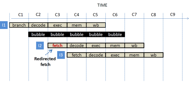
Execution Timeline for control flow instructions: Once I1 is fetched in C1, the pipeline stalls one cycle (C2) to decode the instruction. Then it realizes that this is a control flow instruction (e.g, a beq, jmp, call, etc.) and hence it has to wait for one more clock cycle for the instruction to execute. So, the pipeline stalls for one more cycle (C3) while the control flow instruction executes (stage EXEC). At the beginning of cycle 4 (C4) fetch is redirected to the appropriate PC value and fetching resumes.

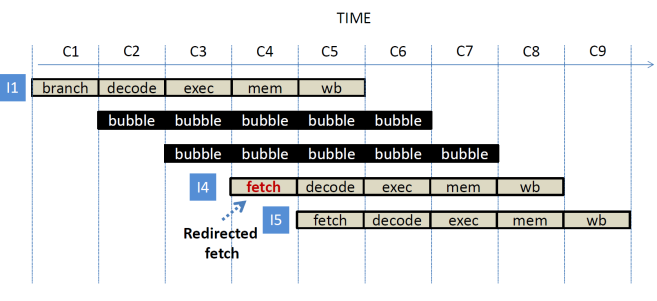
Waiting to determine where to fetch the next instruction induces stalls in the pipeline. In particular, one cycle stalls are induced for all but control flow instructions, and two cycle stalls are induced for control flow instructions.

As we have seen, it is relatively easy to avoid some of the stalls if the pipeline instead guesses what would be the next PC value. Given the current PC the pipeline can easily calculate PC+4 while fetching the current instruction. PC+4 in NIOS II is the PC of the next in memory instruction. This will be the correct next value for the PC in two cases:

1. The current instruction is not a control flow one (e.g., not a branch, jmp, etc.)

2. The current instruction is a control flow instruction which is not taken (e.g., bne r0, r0, somewhere)

This is a straightforward form of control flow prediction or branch prediction coupled with speculative execution. There are two possible execution scenarios:

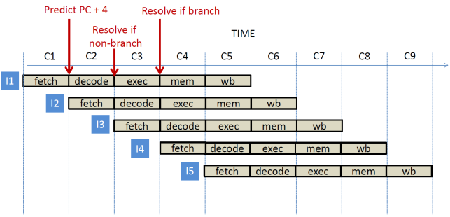
Scenario 1: The fetch stage predicts that the next PC will be PC + 4. If the instruction is not a control flow one that prediction is validated during C2 and becomes available in C3. If this is a control flow instruction and proves not taken, the actual next PC is calculated in C3 during the EXEC stage, and becomes available in C4. Instructions I2 and I3 are both fetched speculatively in cycles C2 and C3, and instruction I2 is decoded speculatively in cycle C3. No stalls are needed and the pipeline can retire one instruction per cycle.

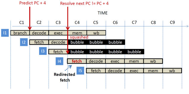
Scenario 2: A branch is fetched in C1 and the fetch stage predicts PC + 4 as the next PC. In cycle C2 instruction I2 is fetched, and in cycle C3 instruction I2 is decoded and instruction I3 is fetched while the branch executes and determines that the current execution path is wrong. In cycle 4, instructions I2 and I3 are squashed inducing two bubbles in the pipeline while the fetch stage is redirected to I4, the correct next instruction after I1.

Since 1 in 5 instructions is typically a branch our pipeline may incur a performance overhead of two bubbles every five instructions. The exact performance lost depends on the instruction mix and on how often branches are taken.

Static Branch Prediction

The prediction that the next PC will be the current PC + 4 is a form of static control flow prediction, or, as it is commonly referred to a static branch prediction. In particular, it is a static, “always not taken” branch prediction method. It is static because the decision does not change at runtime, it is always the same for a particular brand irrespective of what happens during execution. This is the easiest to implement since all it needs is the current PC and a constant. There are other forms of branch prediction that are a bit more tricky to implement. Consider this C code fragment:

     do {
           if (a[i] != 0)
                some computation
           i++;
     } while (i < 100);

In NIOS II assembly this code would be translated to something like this:

     DOWHILE:
          load in r10 a[i]
           beq r10, r0, SKIP
          some computation
     SKIP:
           addi r11, r11, 1
           blt r11, r12, DOWHILE

Where i is in r11 and 100 is in r12. The code has two branch instructions, a beq and a blt. Assuming that most elements of the array would be valid, how would you guess each branch would behave at runtime? How about the beq? Chances are it will not taken most of the time as we will be performing the computation for most array elements. How about the blt? It will execute 100 times, 99 will be taken and once, at the end will be not taken. The simple “always taken” predictor will work well for the beq, but it will fail miserably for the blt. A better static prediction policy is this: “forward not-taken, backward taken”. What does “forward” and “backward” mean? A branch is a forward branch is its taken address is higher than the branch’s address. The beq is a forward branch since SKIP is at the higher, numerically address. A “backward” branch is a branch whose taken address is at a lower address. The blt is a backward branch. Note that the not-taken address is always forward at PC + 4. So, this static branch predictor must determine whether the taken address of an instruction is less than or greater than the current PC. Unfortunately, this is not straightforward for the simple reason that to do so, the actual instruction is needed, the current PC is not sufficient.

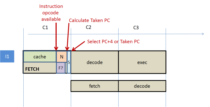
So, how can the “forward not-taken, backward taken” be implemented in practice? One way is to prolong the fetch stage just enough to do the calculation of the taken PC plus a decision as shown below. During the fetch stage, we use the PC to first read the instruction opcode from the instruction cache or memory. Then, while still in the fetch stage, we do the following two things in parallel. Calculate the next PC (typically PC + 4 + sign-ext(Imm16) in NIOS II) while deciding whether the taken PC is forward or backward. The latter decision is easy to make for branch instructions in NIOS II since we just need to look at the sign of the Imm16 offset. A negative offset means a backward branch and a positive offset a forward one (think, is this true for all cases? If not, does it matter that much?). Finally, we can select either the taken and not taken next PC just before the next cycle/stage. The downside of this approach is that the fetch stage and hence the clock cycle must be made long enough to accommodate these actions. Careful instruction set design can help. One has to realize that we do not need to fully decode the instruction. We just need to figure out that this is a branch and what would the taken address. If this is not a branch, we do not care which instruction it is. Moreover, we do not care whether the branch is taken or not. Only what is the taken address. NIOS II’s instruction set encoding is such that determining whether an instruction is a branch is relatively straightforward (a few specific bits in the opcode take a specific value) and the taken address for conditional branches is always PC + 4 + sign-ext(Imm16). Other control flow instructions use different calculations (e.g., jump). We will ignore these for the time being. Suffices to say that we can add functionality to correctly handle these at the expense of additional hardware and most likely lower operating frequency. Alternatively, we can treat those as always not taken accepting a performance hit.

Instead of making the fetch stage long enough to accommodate the calculation of taken PC plus the decision as described, we can instead use a pre-decoding approach. In this approach, pushes the calculation of the taken PC plus the decision as to whether a branch is forward of backward just before the instruction cache. In particular, when a instruction is fetched from main memory, a hardware unit inspects the contents returned from memory, determines whether the instruction is a branch and if so, what is it’s taken address. This is metadata information is stored along the instruction in the instruction cache using extra bits that are invisible to the programmer. Eventually, when the pipeline fetches this instructions it gets both the taken address and whether this is a forward or not branch directly from the instruction cache. Accordingly, it can redirect fetch for the next cycle. This approach essentially moves the taken address calculation and the forward/backward calculation off the fetch stage and pushes it before the instruction cache. Since memory latencies are typically large (in the order of tens or hundreds of cycles) adding an extra cycle to do these calculations does not add much to the latency. Moreover, since the common case is that the pipeline will hit in the instruction cache, this one cycle overhead is paid rarely; once an instruction is pre-decoded and stored in the instruction cache, the pipeline does not to calculate and hence delay for the taken PC and the forward/backward determination. This pre-decoding technique can be used to hide other decoding-related complexities in the pipeline as well.

There are several other static branch prediction techniques. They are rarely used in practice since there are better, albeit more expensive method which we will discuss next.

Generalized Branch Prediction

In general, given a branch instruction, branch prediction entails the following actions:

1. Guessing whether the branch will be taken or not. This is called branch direction prediction, and often, incorrectly referred to as branch prediction.

2. Guess the correct next PC value. This is called target address prediction.

3. Fetching the instructions at the next PC. The is no special term for this.

We will be discussing actions 1 and 2 in more detail next. Action 3 depends on the first two actions and for the most part is straightforward: just fetch the instruction at the predicted PC. We will start with branch direction prediction

Dynamic Branch Direction Prediction

Last Outcome Predition

Static branch prediction makes decisions which do not depend on what happens at runtime. This is pretty naïve. Think of the equivalent in real life. One of the reasons why humans has survived is that they learn and do not repeat the same mistake (at least some of us do). Can the same concept be applied for branch prediction? The idea here is the following: observe and learn. When you first encounter a branch never seen before, just guess something (may be always not taken is good enough). However, once the branch executes once, see what it did and remember that. Next time, when you see the same branch predict that it will do the same as last time. This method will work very well for our previous code example. It will quickly learn that the beq is not taken while the blt is taken. This is called last outcome branch direction prediction, or simply last outcome branch prediction. Here’s an example of how it will behave given the first two iterations of the code above:

ITERATION 1
     DOWHILE:
          load in r10 a[i]
           beq r10, r0, SKIP   FIRST TIME SEEN à PREDICT NOT TAKEN à LEARN NOT TAKEN
          some computation
     SKIP:
           addi r11, r11, 1
           blt r11, r12, DOWHILE FIRST TIME SEEN à PREDICT NOT TAKEN à MISPREDICTION à LEARN TAKEN
     ITERATION 2
     DOWHILE:
          load in r10 a[i]
           beq r10, r0, SKIP   SEEN BEFORE à PREDICT “SAME AS LAST TIME”: NOT TAKEN à LEARN NOT TAKEN
          some computation
     SKIP:
           addi r11, r11, 1
           blt r11, r12, DOWHILE SEEN BEFORE à PREDICT “SAME AS LAST TIME”: PREDICT TAKEN à LEARN NOT TAKEN

and so on…

How well will this predictor work for our example? It will predict the beq correct all the time as long as it is not taken, it will mispredict the blt two times. Once in the beginning for learning that it is taken, and once at the end, when the loop ends where it will predict as taken while the branch will be not taken. The accuracy of the branch predictor is defined as:

# correct predictions / #total predictions

In our example we will have:

100 correct for the beq and 98 correct for the blt out of the 200 in total predictions. So, the accuracy will be 198/200 = 99%

How can we implement this prediction algorithm? There is a price to pay, which amounts to extra storage for “remembering” what happened last time we saw a particular branch. Specifically, for each branch that we encounter, we need to remember two things: 1. Which branch it was; that is its PC value. 2. Which direction it went, taken or not taken (recall, for the time being we are only interested in the taken/not taken decision, we will discuss predicting the target address later on).

Implementing last-outcome prediction

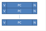
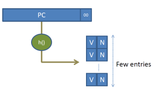
One straightforward implementation of this technique is to create a prediction table which is an associative table, or a content addressable memory, with three fields: (1) A PC value, (2) a single bit encoding not taken as 0 and taken as 1, and (3) a valid bit indicating whether this entry contains valid information or not. We can create a table containing such entries. Ignore the issue of how many we need for the time being. In the beginning all entries are “empty” which is signified by having their valid bits at 0. Once a branch is fetched, we use its PC and compare against all entries (I know this appears, expensive, hold on, we will simplify soon). If there a match we can use the information from the taken/not taken bit. In the beginning all of the entries are empty, so there will be no match, and hence we will fall back to a default prediction, say PC +4 which is easy to implement. Once the branch executes, we can then see what direction it took and if necessary allocate an entry for it in our prediction table. Next time, once we encounter the same branch, we will look it up using the same PC and find the information about what it did last time. If we are lucky, history will repeat itself, and the prediction will be correct. Once the branch executes, we can go back and update the prediction information. This way the predictor can adjust at runtime in response to the branch’s behavior. This is why this is a dynamic predictor.

The implementation described might be straightforward to understand but is expensive. In particular, if we need one entry per possible branch, we will need 2^32/4, that is 2^30 or 1G entries for the 4G address space of NIOS II, since a branch can appear anywhere in memory. Each entry would contain a full PC (that’s 4 bytes) plus two more bits. That is a lot of storage and more than our main memory. But wait, if we are going to have an entry for each possible PC then we do not need to store the PC value in it. Starting from a PC, we can simply index the corresponding prediction table entry and get the valid and prediction bits. So instead of having a table like this:

We can have a table like this:

The problem is that this table still needs to have 1G entries. While each entry is 2 bits wide, in total we are still looking at 256Mbytes of storage. That is still a lot. What can we do to reduce its size?

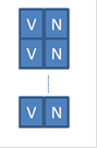
First, let’s recall that we are predicting. That is, we can be wrong or right and the machine will still execute the program correctly. Being wrong just reduces performance. So, how about we have branches share table entries? This can be done with a hash function. So instead of having a table with 1G entries that is directly indexed by all relevant bits of the PC like this:

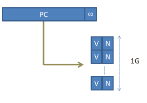
We can have a smaller table with as many entries we can afford which is indexed using a hash function as in this:

For example, the table can have 2K entries only. The hash function needs not be something overly complicated. For example, for a 2K entry prediction table, we can use just the lower 11 bits (after ignoring bits 1 and 0 which are always 0 as the instruction needs to be aligned at a 4-byte granularity).

Once we have limited the number of entries, we will have collisions, that is different branches will map onto the same prediction table entry. This is called aliasing. Aliasing can be destructive or constructive. That is, if the two aliasing branches have opposite behavior they will interfere reducing prediction accuracy. If they have the same behavior they will reinforce each other and accuracy may improve when the decision changes (observing the change for one branch will be enough to correctly predict the changed behavior for the other).

Finally, since we no longer have a PC, many different branches may map to each entry, and since we are predicting anyhow, what is the point of having valid bits? We can simply drop them and have a simple prediction table as follows:

The Problem with Last-Outcome prediction

Last-outcome prediction is nice, but it is like a bad politician. Anyway the wind blows it goes. That is, it quickly changes its mind. Again, going back to our do-while loop example think what would happen if that loop were to execute multiple times. The first time the loop executes, our predictor will quickly learn that the blt is taken. At the 100^th iteration however, our predictor will fail to predict that this is the last iteration and predict taken. It will misspredict as the loop will exit. Immediately, the prediction bit will be updated. Next time the loop runs, at the end of the first iteration, the predictor will miss-predict not taken. It will adjust to predict taken and then correctly predict the rest 98 iterations. Again at the 100^th will miss-predict.

Adding Hysterisis – Two bit predictors

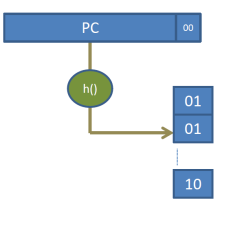
A solution to this is to add some hysteresis in the prediction mechanism. That is, we will still allow the predictor to change its mind, but it will do so with some resistance. A simple, hysteresis mechanism is a 2-bit up/down saturating counter which operates as follows:

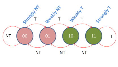
Each prediction table entry now has two bits which are updated according to the diagram above. The table looks as follows:

There are four possible values which take the following meaning:

1. 00: means strongly biased toward not taken à predict not taken

2. 01: weakly biased toward not taken à predict not taken

3. 10: weakly biased toward taken à predict taken

4. 11: strongly biased toward taken à predict taken

The diagram shows how the counter changes value according to the actual direction of the branch. The labels on top of the arrows show the actual branch outcome. For example, assuming that the current value is 10 the predictor is weakly biased toward taken and will predict taken. If the actual direction proves to be taken, the predictor will be updated to 11 and will become strongly biased toward taken. If the direction is not taken, the predictor will be updated to 01 changing its decision for time and becoming weakly biased toward not taken.

In our loop example, let’s assume the predictor for blt is initially weakly biased toward taken. The first loop iteration will correctly predict taken and will then move to be strongly biased toward taken. For the next 98 iterations it will predict taken and stay at 11. For the 100^th iteration it will miss-predict and move to 10, weakly biased toward taken. Next time the loop starts executing it will correctly predict the first iteration and thus avoid the extra miss-prediction that the last-outcome predictor suffered. While for a loop that iterates 100 times the difference in accuracy is minor, for shorter loops avoiding that extra miss-prediction is significant.

The two bit saturating counter is an example of a confidence mechanism. We can think of many others. For example, we can use a 3-bit saturating counter in order to add more hysteresis in changing prediction direction. Such predictors are called bi-modal.

The problem with bimodal predictors

Let us now consider these nested loops:

i = 0;
do {
           j = 0;
     do {
           some calculation
           j++;
     } while (j < 2);
     i++;

} while (i < 3);

The equivalent NIOS II code would look something like this:

     movi r18, 3     # max i
     movi r19, 2     # max j
     movi r8, 0      #i = 0
DOi:
     movi r9, 0      # j = 0
DOj:
     some computation
     addi r9, r9, 1
     blt r9, r19, DOj #J branch
     addi r8, r8, 1
     blt r8, r18, DOi # I branch

When this code runs we will see the following pattern for the “J branch”:

T T NT T T NT T T NT

Our 2-bit confidence counter will struggle with this. Assuming that it starts say from 10 (weakly taken), it will make the following predictions:

T (11) T(11) T(10) T(11) T (11) T(10) T(11) T (11) T(10)

It will miss-predict three times (the numbers in parentheses show the predictor state after each prediction is resolved).

However, the pattern that the “J branch” exhibits is fairly regular: two taken followed by one not taken. Can we design a predictor that can predict this kind of patterns?

Pattern-Based Predictors

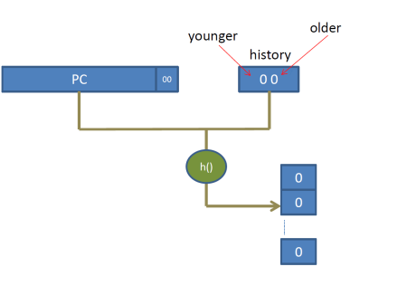
The idea behind pattern based branch predictor is to associate a prediction not just with a particular branch but also with a history of other related events. In particular, we can associate a prediction with both a PC and a series of recent branch outcomes. This is pattern-based prediction. In this prediction a shift register is introduced. Each bit corresponds to the direction taken by the N most recent branches. Each time a branch is predicted, we shift the register by one bit to the right and add an extra bit with the direction predicted for the current branch. To make things easy to understand, let’s pretend that the only branch that we were to observe at runtime was the J branch above. How will the prediction proceed? Let’s assume that we had a 2 bit history register and that initially the register is all zeroes corresponding to NT. Let’s see at three invocations of the inner j loop above. In this example assume that the only PC that will access the prediction table is the “J branch” and that there are enough entries to store all possible patterns. When indexing the prediction table we use both the PC and the pattern as specified by the history register. This can be done for example by concatenating the two (this is called a gselect predictor) or by hashing them together somehow through say some xor function (this is called gshare):

Here’s what happens for the first time the J loop executes:

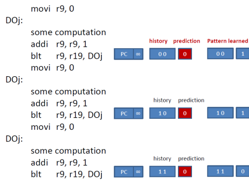
The first time the J branch executes, the history register contains 00 and the prediction is NT. This is assuming that all entries in the prediction table are initialized to NT. The predictor miss-predicts and when the J branch executes eventually, the predictor learns that the history pattern 00 leads to T. The history register is updated to 10, since the last branch that was since was taken. The second time the branch executes, it again resorts to the initial value provided for the history pattern 10, which incorrectly set to NT. It miss-predicts and learns that 10 leads to T instead. The history register is now 11 since the last two times J was taken. The third time, the predictor correctly predicts NT just by luck as the default initial value is NT. It also learns that 11 leads to NT. History is updated to 01, since the last branch was not taken and the previous to last was taken. So far our predictor has learned three patterns: 00 à T, 10 àT, and 11 à NT.

Let’s now see what happens when the J loop executes again:

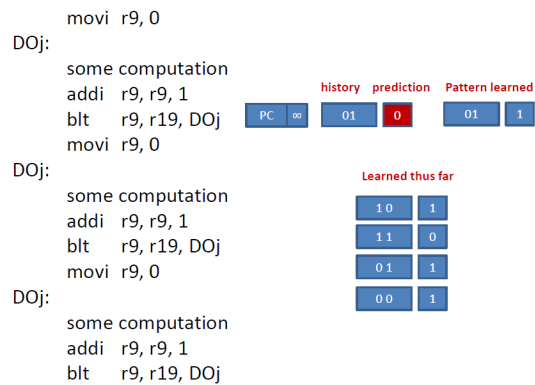
The 4^th time branch executes, there is no information in table for the current history pattern of 01 and hence we get the default NT which proves wrong. The predictor, however, learns that 01 leads to T. At this point the predictor has learned the four patterns shown in the diagram above. From this point on, as we shall see the predictor will predict all J branches correctly 100% of the time. Here’s what happens next.

History is now 10. The predictor has learned that 10 leads to 1 which is the correct prediction. History now becomes 11. The predictor for the next branch sees that 11 leads to 0 and correctly predicts that the next J branch will be not taken. History now becomes 01. Let’s see what happens if the J loop is invoked again:

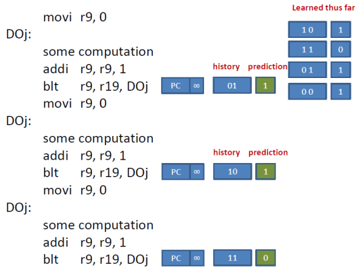
At this point, you should be able to follow the example and to see that our predictor correctly predicts all instances of the J branch since it learned the three possible history patterns, 11, 01, 10.

In the example we discussed we assume that the predictor table stores just a single bit for each prediction. However, we can still use the two-bit saturating counter for hysteresis. Most processors today would implement a pattern based predictor. There are quite a few variants depending as to whether the history register is shared among all branches, and whether there are separate prediction tables per branch. In practice, the history register is shared and all branches access a single table using a hash of the PC and the current history. The exact history length that works best varies within and across applications and is determined experimentally. There are even methods that adjust the history length at runtime using a sample and run approach. In this approach, we start with one length and run for a while measuring accuracy. After say 10K cycles we adjust the size and run again. After 10K cycles we compare the accuracy with the new history length versus the one used before. We pick the best and move along with that. This process of adjust continues for ever.

The problem with pattern based predictors.

As the example has shown, it takes a while for a pattern predictor to learn how a branch behaves. It may be more capable than a simple bi-modal predictor but it takes a while to do so and uses many entries. In summary, bi-modal is a fast learner but it can only learn so much, gshare/pattern is clever but it takes a while to light the fuse. Enter tournament predictors. These predictors try to get the best of both worlds. They run in parallel say a bi-modal and a gshare predictor and then try to pick the best of the two:

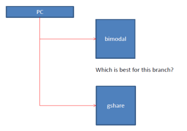
How does it pick which is best? It predicts using another predictor which is often another bimodal:

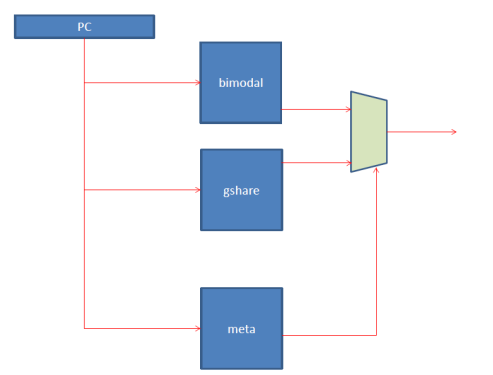
The first two predictors observe the branch stream, PCs and taken or not taken and operate as we described. The third, meta predictor observes the other two and in particular whether they are wrong or right. It adjusts its decision toward the one that is right (breaking ties either way probably preferably toward the bimodal which is more space efficient). Most high-end processors today implement some variant of this tournament predictor.

Rush job

Branch predictors operate under very strict time constraints. They have to make a decision within a single clock cycle in order to be able to continuously feed the pipeline with new instructions. Branch prediction accuracy can increase considerably if larger tables are used since this reduces aliasing and allows us to learn more patterns. However, larger tables are slower. As a result, processors are often use very small predictors that are not as accurate as we would wish. If someone is willing to pay the price, there is a better solution where two predictors operate in parallel. The first is a fast that operates within a single clock cycle. The second is a much larger, overwriting predictor that may take multiple cycles to make a prediction. For example, in our 5-stage pipeline, the overwriting predictor may take two cycles and produce a better prediction by the end of decode:

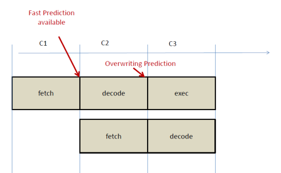
If the overwriting predictor agrees with the fast predictor nothing changes, however, if it disagrees, the pipeline may be flushed and fetch redirected right now. In our five stage pipeline, this may save just one cycle which doesn’t seem much. However, if you think of a modern OOO processor which is deeply pipelined and has many outstanding branches, it make take several 10s of cycles before the branch is resolved, so a more confident prediction may be better.

Predicting the Target Address

So far, we were concerned with predicting whether the branch will be taken or not. If it’s taken it would be nice to know where it goes to. We said that one option is to calculate this at the fetch stage at the cost of making the clock cycle slow enough to accommodate this calculation. An alternate approach is to predict the target address. A simple last-outcome predictor can be used here as well. That is, the first time we see a branch we take our losses and do not predict the taken address. However, once the branch executes and we see which is the taken address we store it in in a separate Branch Target Buffer table (BTB). Next time around, we encounter the same branch we look it up in the BTB using just its PC where we will find its target address. To avoid aliasing we can tag each entry with the PC that it corresponds to:

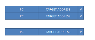
This BTB works very well for NIOS II’s branches since the taken address does not change at runtime. It can also be used for Jump instructions. It will work reasonably well for indirect branches such as those using a register for the target address (used in switch statements and function pointers for example, or to implement virtual functions in C++). More advanced techniques have been proposed to increase accuracy for indirect branches where, for example, a history pattern is used to associate different possible target addresses with different execution paths.

Putting it all together

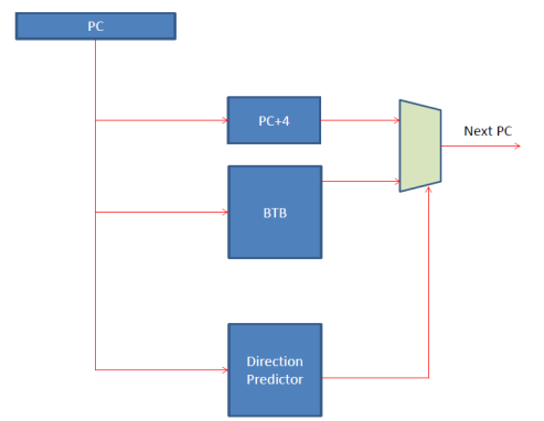
In summary, the fetch stage contains a branch direction predictor and a Branch Target Buffer which operate in parallel. The branch direction predictor provides a taken/not taken prediction and the BTB provides the taken address. In parallel we also calculate the fall through address (PC + 4) and select between that and the one provided by the BTB based on the direction prediction:

Calls and Returns

Call and returns are very frequent and foil the BTB. In particular, the BTB will correctly predict calls since their target address does not change, however, it will fail to predict returns since the return address varies depending on where the call was made from; the same ret instruction may return to different addresses. However, where the ret will return is known at call time. Since these are frequent instructions a specialized prediction mechanism is used. Specifically, a hardware stack is used. When fetch encounters a call instruction it pushes on the stack PC+4 which is the return address for the call. When a return is encountered, fetch pops an address from this hardware stack. The hardware stack is not visible to the programmer and works perfectly as long as the call depth does not exceed its capacity.

Avoiding Control Flow when we can

Consider the following if statement:

If (error != 0) error_handle();

Assuming that errors are rare the above code will rarely jump into error_handle(). Branch prediction will correctly learn this and avoid stalling. Now consider this branch:

If (a[i] < threshold) a++; else b++;

What the branch will do is completely depending on the values of a[i]. We may get a runtime pattern that is easy to predict or we may get one that will foil our predictors. Is there an alternative? Another possibility is to use predicated instructions. These instructions take the following form:

cond register: some instruction

Where cond register is a reference to a single bit register. If the value of that register is 0 the instruction converts on the fly into a no op (does nothing), otherwise if the condition register is 1, the instruction executes normally.

Let’s look at the code we had before. Here’s how it is implemented in conventional NIOS II machine language:

                Load a[i] in r8
                blt r8, r9, THEN                # r9 holds threshold
ELSE:
                addi r10, r10, 1                   # b++
                br            DONE

THEN:
addi r11, r11, 1 # a++
DONE:

A pipeline will struggle with the blt instruction trying to predict a data dependent pattern. In a hypothetical predicated NIOS II variant we would have this:

                Load a[i] in r8
                cmplt c0, r8, r9 # condition register c0 = r8 < r9
c0:          addi r10, r10, 1
!c0:         addi r11, r11, 1

The first c0: addi writes into r10 only if c0 is TRUE while the !c0: addi writes into r11 only if c0 is FALSE. In this code there are no branches so nothing to predict and no possibility of miss-prediction which is great. However, notice that no matter what one of the instructions will be converted to no op. So, we will effectively have one bubble in the pipeline. This is the price we pay with predication. This is less of a concern for if-then constructs as it is not always the case that we will see no ops. A commonly used instruction set that provides prediction is that of ARM. GPUs are also implementing predication. General purpose processors usually implemented a poor-man’s predication alternative in the form of a conditional move. For example, in a hypothetical NIOS II implementation we could have:

cmov r10, r11, r12

which does r10 = r11 only if r12 is non-zero (TRUE).